Blogger develops system that geolocates videos by background aircraft noise with accuracy to within 100 meters

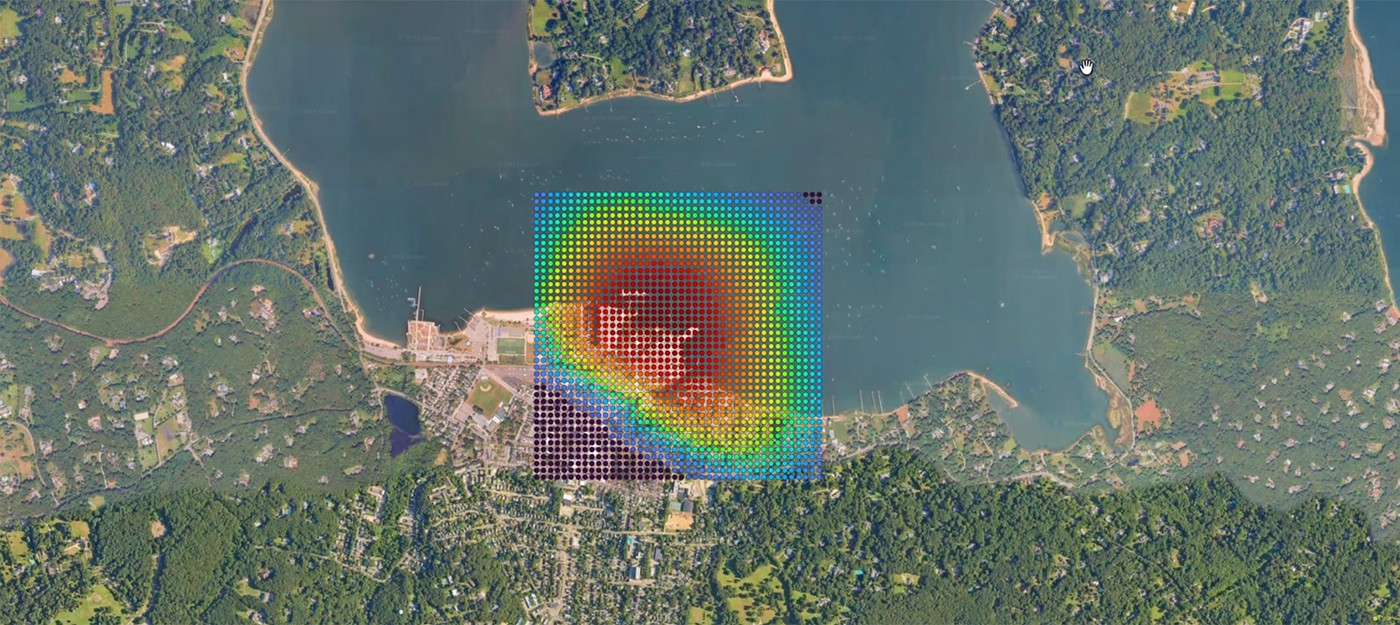
YouTuber colsto, who specializes in geolocating photos and videos, showed how to pinpoint where a clip was filmed using the sound of passing planes. A security camera recording in which nothing changes in frame was enough. The only starting data were the recording date, September 8, and the fact that the video was shot somewhere in the continental US.
The blogger had already tried geolocation using rolls of thunder. Thunder carries over long distances and passes easily through walls, but that method was accurate to only about 5 km – good for a city and a rough district at best. The new approach keeps the same advantages and narrows the search area to around a hundred meters.
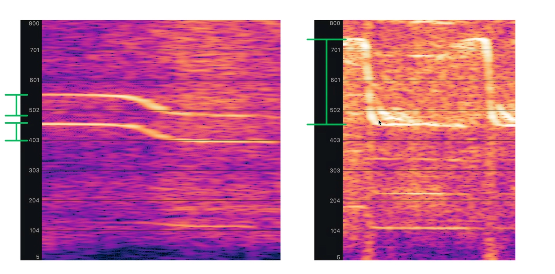
The key was the Doppler effect. A plane flyover is barely audible in the recording, but on a spectrogram, with time on the horizontal axis and frequency on the vertical, a characteristic Doppler curve appears once the right frequency range is magnified. The camera footage contained two such curves from propeller planes, 920 seconds apart.
Fair warning, this is insanely powerful, but it takes a lot of complicated work. It took months and more than 5,000 lines of code to build. I worked with 50 GB Parquet files, 3D physics modeling, digital elevation models of an entire country, and a lot more.
The search relied on ADS-B data, which nearly every aircraft in the sky broadcasts, including coordinates, speed, altitude, and other parameters. The blogger spent several hours pulling every flight over the US on September 8 through Python, then used the ICAO aircraft type table to filter out known jet models, since the sound in the recording clearly came from a propeller plane.
Next, a grid of points with 200-meter spacing was built within a 10 km radius around each flight path. For every point, the script calculated the time of closest approach, when the plane sounds loudest. Sound delay was factored in too – it takes several seconds to reach the observer, and it travels along the slanted distance rather than the horizontal one.
Another catch surfaced here. ADS-B reports altitude above sea level, not above ground, so calculating the real distance required a digital elevation model with the height of every grid point. Only then could the search begin for places where a plane was audible and a second one passed 920 seconds later.
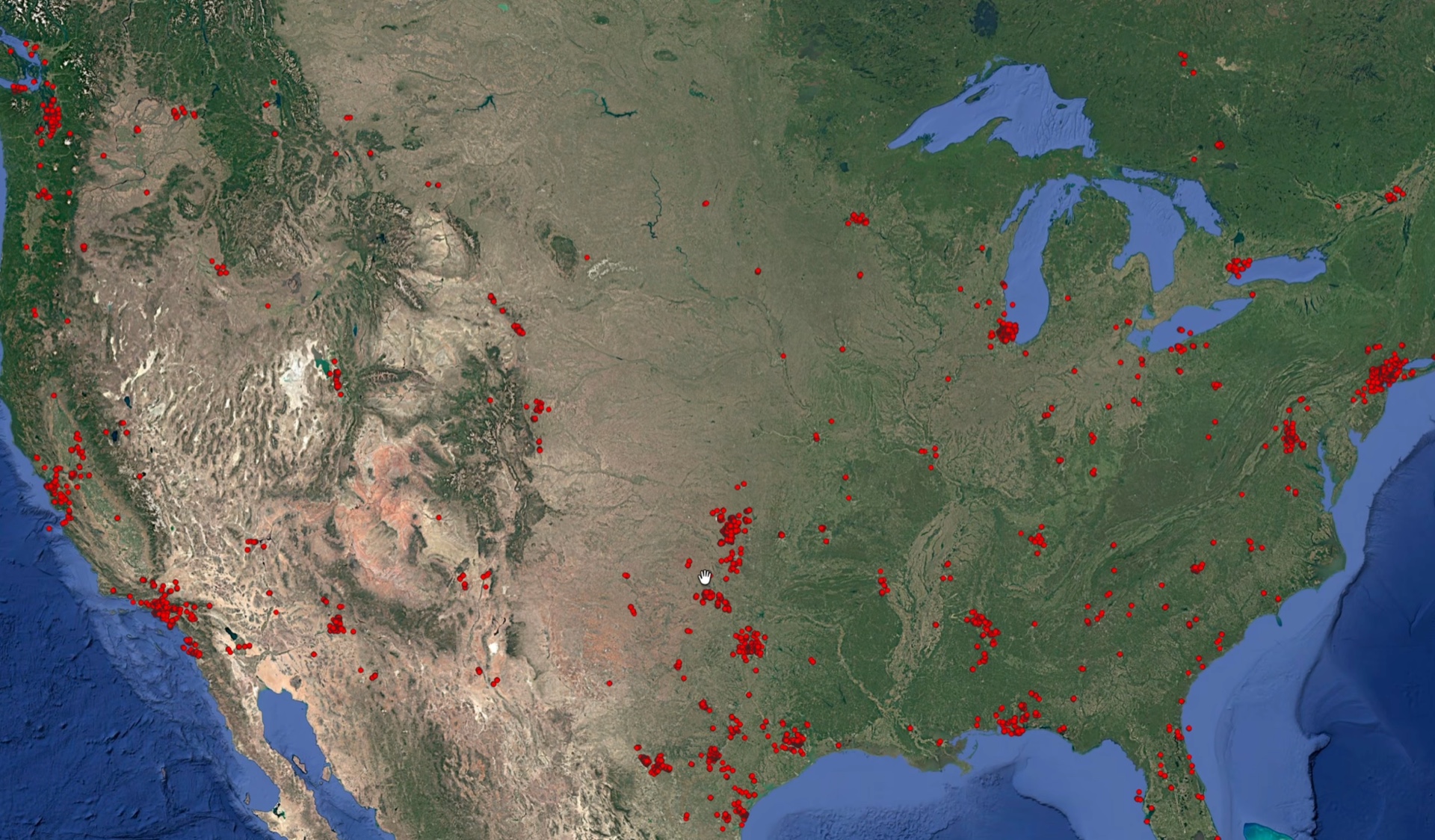
Even on a test area covering less than 0.05% of the continental US, about 35,000 points met that condition.
The shape of the Doppler curves helped narrow things down. For uniform straight-line motion, only two parameters define it:
the plane speed sets the size of the frequency drop
the distance to the observer at the point of closest approach sets how sharply that drop happens
For the first flyover, the speed came out to about 100 m/s. After filtering by speed and distance, roughly 73,000 points remained, but most clustered near airports, where heavy traffic raises the odds of a chance match.
Silence turned out to be useful as well. Between the two flyovers, the recording has almost 15 minutes without a single plane audible, which doesn't happen near a major airport. A filter for the absence of other flyovers cut the number of candidates to about 15,000.
That's where the simple signals ran out, and the blogger moved on to the main part. The real curves in the recording didn't match the ideal shape, because planes change course, speed up, slow down, and shift altitude. Instead of trying to reconstruct a trajectory from the spectrogram, colsto simulated which Doppler curve each candidate would hear given the actual geometry of each flight.
The model needs radial velocity – the speed at which the plane moves directly toward or away from the observer. If a plane flies straight at a person, radial velocity equals its full speed, and if it passes directly to the side, it is nearly zero and there is no Doppler effect. That value goes into the Doppler formula along with the speed of sound and the source's base frequency.
The blogger pointed out one mistake that would have wrecked the search entirely. The frequency an observer hears at a given moment depends on the speed of the plane not at that moment, but at the moment the sound that reached the observer was emitted. Simply shifting the curve in time doesn't fix it – the wrong approach produces a curve of a completely different shape.
Each simulated curve was overlaid on the spectrogram, and the brightness of the pixels under it was summed. Small errors in timing and base frequency were compensated for by testing values within a few seconds and hertz. The position of the second flyover relative to the first was locked in by the real flight geometry, so a wrong candidate inevitably got a low score.
For an accurate estimate, the grid had to be refined to 100 meters – with 200-meter spacing, the correct point could sit 141 meters from the nearest node and score poorly. Calculations for 30,000–40,000 points demanded huge computing resources, and without prefiltering, running them across the entire US in a single day would have been impossible.
The top candidate scored 20.48 against about 15 for the nearest competitor, and its simulated curves fully covered the real ones on the spectrogram. Other options matched the first flyover reasonably well, but the second one clearly diverged.
Then the blogger ran a second experiment. He took just one minute of audio with a barely visible curve, one that can't be heard even when listening for it, and provided only the recording time, 20:37 UTC. The search again covered the whole US, and the same point at latitude 40.8735 came out on top by a clear margin.
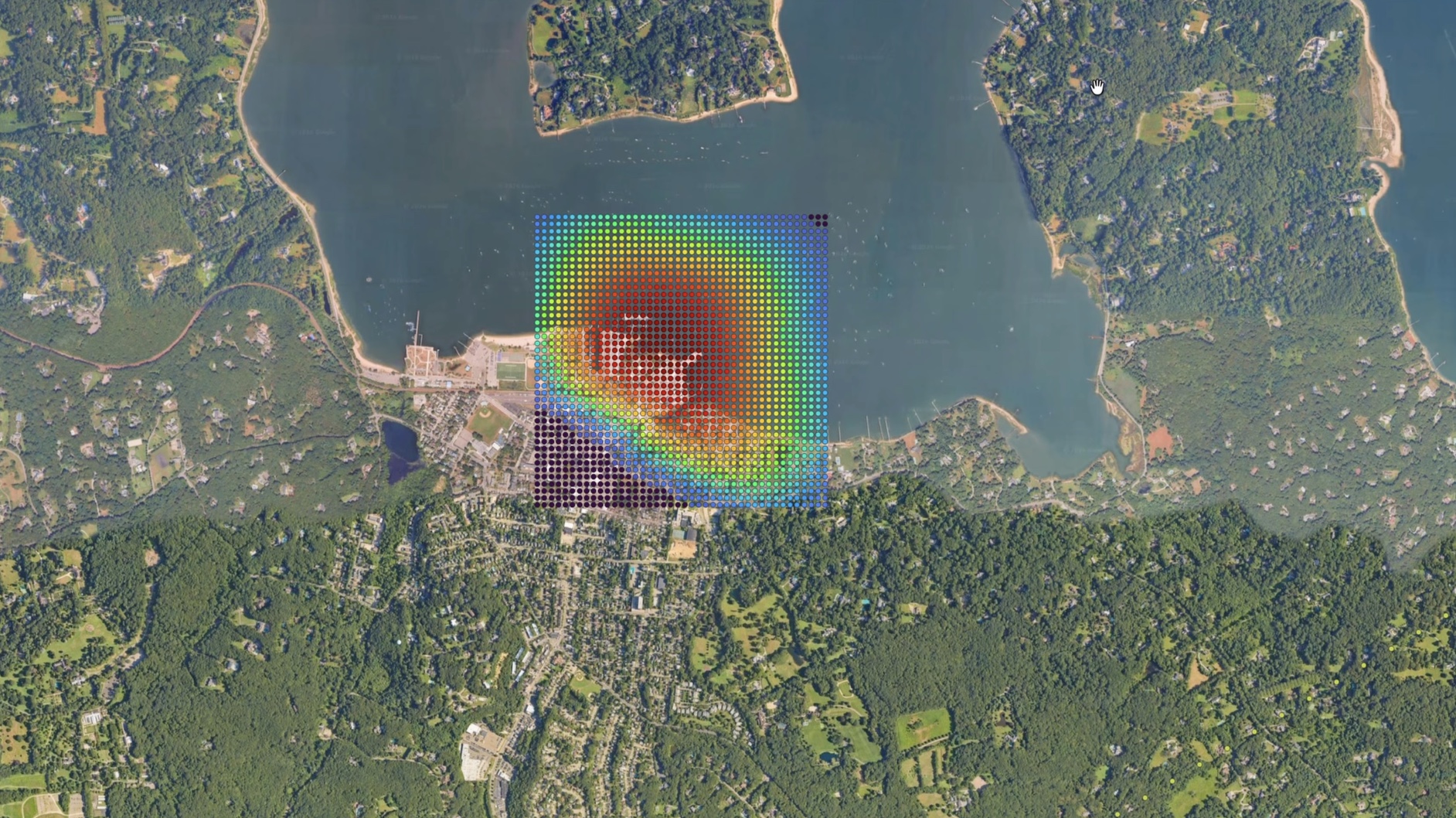
According to colsto, it's enough for just one of the parameters to be good. In the first case, the location and time were unknown, but there were two flyovers, while in the second there was only one flyover, but the time was known exactly. If at least the city is known, which is about 0.01% of US territory, the timing requirements drop sharply, and there's no need to know the minute, the hour, or even the day of filming.
The blogger ran the final check in Google Street View. The calculated point turned out to be on the shore of a body of water, and the distinctive silhouette of a tree line with a V-shaped crown helped find the right angle. At the top of a pole at that spot hung the very same security camera.

The blogger also tested ways to defend against the method, and most of the obvious options failed. A high-pass filter cuts out a noticeable part of the human voice, since Doppler curve frequencies nearly coincide with speech. Also, after exporting such a recording to MP3 and boosting all frequencies, the curve reappeared on the spectrogram.
Drowning out the signal with talking didn't work either. During recording, colsto spoke for 15 seconds with a JBL speaker on the other side of the room playing a Doppler curve, and the curve still survived on the spectrogram. It also survived a phone call, despite audio compression and noise suppression.
We pinpointed the recording location to within a couple hundred feet from one minute of audio where you can't even hear the plane. And these flyovers happen all the time. These frequencies pass through walls. This could be in any video you've ever filmed.
Only editing cuts, which strip the analysis of the time interval between flyovers, and additional noise suppression actually help. The blogger added that he isn't trying to spread panic – the chance that someone could and would run such an analysis is small, and there are a hundred simpler ways to find a person.
colsto sees the main practical use of the method in investigations where a recording contains no visual clues at all.
According to the developer, the video is educational and relies on open data, and the blogger chose not to publish the code and tools.